Business impact:
- The fashion industry is in the transition stage from traditional advertisement to computer-vision based the recommendation system for online advertising;
- It is critical to building a fashion classification system to help the customer identifies different fashion categories from social media, blog, or his/her own pictures.
- The virtual assistant is able to analyze a customer’s preference and recommend to the related fashion clothes.
In this project, I was trying to classify different fashion styles (totally 60000 training pictures and 10000 testing figures) on the category of 10 using deep learning approach. The dataset is from: http://mmlab.ie.cuhk.edu.hk/projects/DeepFashion.html
The classification types are:
- 0 => T-shirt/top
- 1 => Trouser
- 2 => Pullover
- 3 => Dress
- 4 => Coat
- 5 => Sandal
- 6 => Shirt
- 7 => Sneaker
- 8 => Bag
- 9 => Ankle boot
Let’s load the dataset and create training and testing array
Pfashion_train_df = pd.read_csv('fashion-mnist_train.csv',sep=',')
fashion_test_df = pd.read_csv('fashion-mnist_test.csv', sep=',')

training = np.array(fashion_train_df, dtype = 'float32')
testing = np.array(fashion_test_df, dtype='float32')
Plot some examples from the training dataset:
W_grid = 10
L_grid = 10
fig, axes = plt.subplots(L_grid, W_grid, figsize = (20,20))
axes = axes.ravel()
n_training = len(training)
for i in np.arange(0, W_grid * L_grid): # create evenly spaces variables
    index = np.random.randint(0, n_training)
    axes[i].imshow( training[index,1:].reshape((28,28)) )
    axes[i].set_title(training[index,0], fontsize = 8)
    axes[i].axis('off')
plt.subplots_adjust(hspace=0.4)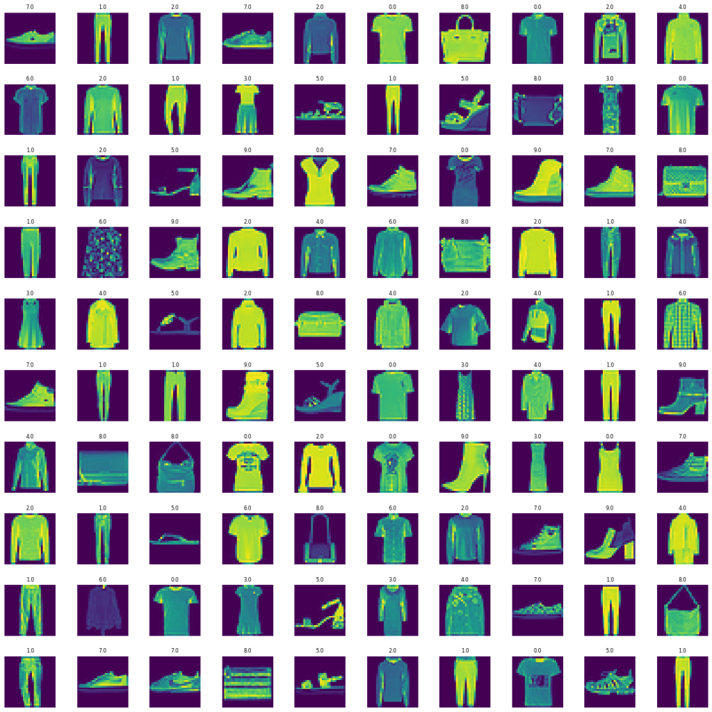
It is better to normalize each figure to avoid overfitting, then split to train and test sets:
X_train, X_validate, y_train, y_validate = train_test_split(X_train, y_train, test_size = 0.2, random_state = 12345)Start to build a convolutional model on Keras:
model2 = Sequential()
model2.add(Conv2D(32, (3, 3), activation='relu', padding='same', name='conv_1',
                 input_shape=(28, 28, 1)))
model2.add(MaxPooling2D((2, 2), name='maxpool_1'))
model2.add(Conv2D(64, (3, 3), activation='relu', padding='same', name='conv_2'))
model2.add(MaxPooling2D((2, 2), name='maxpool_2'))
model2.add(Conv2D(128, (3, 3), activation='relu', padding='same', name='conv_3'))
model2.add(MaxPooling2D((2, 2), name='maxpool_3'))
model2.add(Conv2D(128, (3, 3), activation='relu', padding='same', name='conv_4'))
model2.add(MaxPooling2D((2, 2), name='maxpool_4'))
model2.add(Flatten())
model2.add(Dropout(0.25))
model2.add(Dense(512, activation='relu', name='dense_1'))
model2.add(Dense(128, activation='relu', name='dense_2'))
model2.add(Dense(10, activation='sigmoid', name='output'))
model2.compile(loss='sparse_categorical_crossentropy',optimizer=Adam(lr=0.001),metrics=['accuracy'])
epoches=50
history = model2.fit(X_train,y_train,batch_size=32,nb_epoch=epoches,verbose=1,validation_data=(X_valid,y_valid))

=======================================================================================
Epoch 48/50
48000/48000 [==============================] - 19s 390us/step - loss: 0.0523 - accuracy: 0.9855 - val_loss: 0.4039 - val_accuracy: 0.9193
Epoch 49/50
48000/48000 [==============================] - 19s 395us/step - loss: 0.0513 - accuracy: 0.9836 - val_loss: 0.4007 - val_accuracy: 0.9211
Epoch 50/50
48000/48000 [==============================] - 19s 396us/step - loss: 0.0508 - accuracy: 0.9848 - val_loss: 0.3770 - val_accuracy: 0.9197
#Evaluation...
evaluation = model2.evaluate(X_test, y_test)
12000/12000 [==============================] - 1s 104us/step
Test accuracy = 0.9197499752044678#Testing....
predicted_classes = model2.predict_classes(X_test)(It may be necessary to construct a deeper model to better classify each figure, I will show other network architecture in other projects)
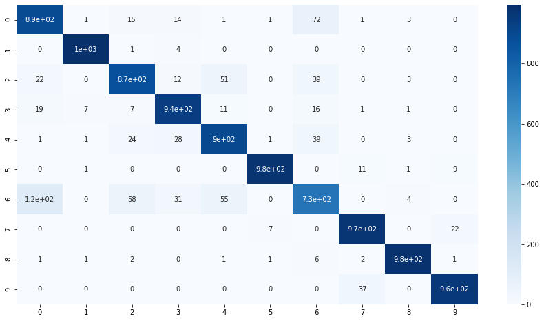
Some parameters will be needed to finetuned, such as batch size, kernel size, the number of epoch and etc. After final prediction, the confusion matrix can be printed out as:
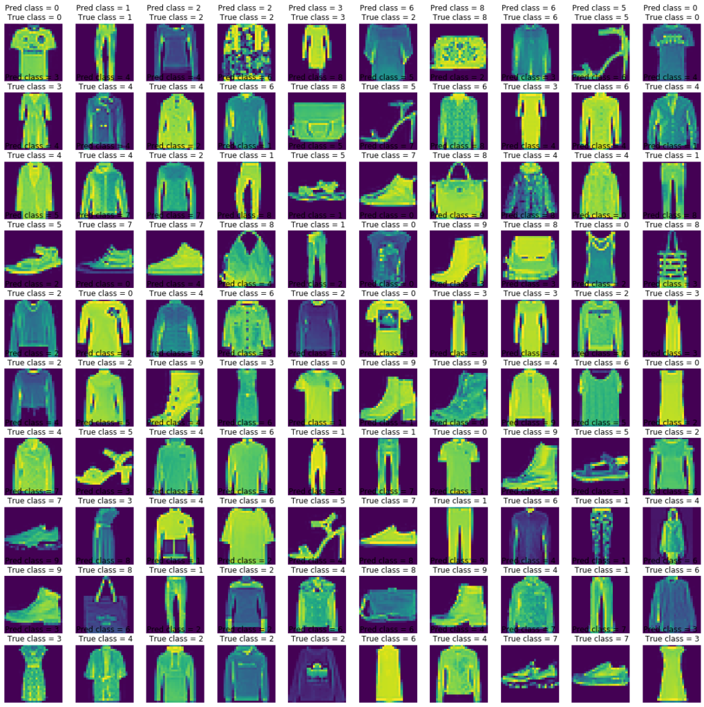
The following plot shows the prediction of labels towards each fashion figure:
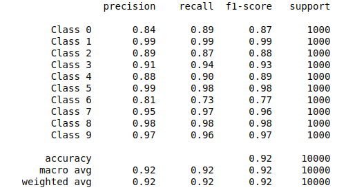
Here I plot the classification report, which includes precision rate, recall rate, f1-score for evaluation: